Functions to directly access the database ressources
database-access-functions.RmdIntroduction
The ratlas package provides functions to interact with
Biodiversité Québec’s database Atlas. For most use cases,
ratlas get functions such as get_taxa,
get_observations, get_datasets, etc should be
used, as they are designed to be more user-friendly. However, in some
cases, it is useful to directly access the database ressources.
This vignette describes how to do so using low-level functions
db_read_table and db_call_function, on which
ratlas get functions are based and is intended for advanced
users.
Atlas database
Atlas database is a PostgreSQL database. It contains several tables, views, materialized views, functions, etc. Data is stored and made available through those resources. While table store data, views and materialized views behaves as tables and are used to store queries, and functions are used to perform operations on the data. They are organized by different schema, each of them representing a different application layer of the database. The following schemas are available:
-
public: Raw biodiversity data is stored here in tables such asobservations,taxa_obs,datasets,variables,efforts, etc. This schema is relational, as joins between tables are required to retrieve data. Data may be protected by access rights and require authentication to be accessed through a token (see README). -
api: This schema contains views and functions that are used to access data from thepublicschema. It performs joins between tables, and returns data in a more user-friendly format. This schema is used by theratlasread/call functions. Data may be protected by access rights and require authentication to be accessed through a token (see README). -
atlas-api: This schema contains tables, views and functions required for the operation of the ‘atlas web portal’. All displayed information and summary statistics are computed from resources in this schema. Data at this layer is not protected by access rights and can be accessed without authentication.
Documentation for tables and functions are made availabe in atlas-db repository documentation.
Reading tables and views data
The db_read_table() function is used to read data from a PostgreSQL table. It takes several arguments, including the name of the table, the schema that the table belongs to, and the authentication token that is required to access the database.
Here’s an example of how to use the db_read_table() function to read data from a table named “taxa_obs” in the “public” schema:
library(ratlas)
# Added a limit of 100 to simplify the process
# Remove the limit argument if you want the whole table
data <- db_read_table("taxa_obs", schema = "public", limit = 100)
The db_read_table() function returns a data.frame object containing the data from the table. The data.frame columns are named after the table columns. The data.frame row names are the row numbers of the table.
Filtering data using column values
The db_read_table() function also allows you to filter the data that
is returned by specifying additional arguments. For example, you can use
the ... argument to specify a filter condition:
data <- db_read_table("taxa_obs", schema = "public", id = 1)

# Or

data <- db_read_table("taxa_obs", schema = "public", scientific_name = 'Acer saccharum')
head(data)
#> # A tibble: 2 × 8
#>       id scientific_name authorship rank    created_at   modified_at modified_by
#>    <int> <chr>           <chr>      <chr>   <chr>        <chr>       <chr>
#> 1   7278 Acer saccharum  Marsh.     species 2021-11-23T… 2021-11-23… postgres
#> 2 939205 Acer saccharum  Marshall   species 2024-01-07T… 2024-01-07… vbeaure
#> # ℹ 1 more variable: parent_scientific_name <chr>

# Using a list of values

data <- db_read_table("taxa_obs", schema = "public", id = c(1, 2, 3))
head(data)
#> # A tibble: 2 × 8
#>      id scientific_name     authorship rank   created_at modified_at modified_by
#>   <int> <chr>               <chr>      <chr>  <chr>      <chr>       <chr>
#> 1     1 Prunus pensylvanica L. fil.    speci… 2021-11-1… 2021-11-19… vbeaure
#> 2     2 Sorbus americana    Marsh      speci… 2021-11-1… 2021-11-19… vbeaure
#> # ℹ 1 more variable: parent_scientific_name <lgl>

data <- db_read_table("taxa_obs", schema = "public", scientific_name = c('Acer saccharum', 'Acer rubrum'))
head(data)
#> # A tibble: 4 × 8
#>       id scientific_name authorship rank    created_at   modified_at modified_by
#>    <int> <chr>           <chr>      <chr>   <chr>        <chr>       <chr>
#> 1   7279 Acer rubrum     L.         species 2021-11-23T… 2021-11-23… postgres
#> 2 928393 Acer rubrum     L.         species 2024-01-07T… 2024-01-07… vbeaure
#> 3   7278 Acer saccharum  Marsh.     species 2021-11-23T… 2021-11-23… postgres
#> 4 939205 Acer saccharum  Marshall   species 2024-01-07T… 2024-01-07… vbeaure
#> # ℹ 1 more variable: parent_scientific_name <chr>
Selecting columns and limit the number of rows
The limit and select arguments can be used to limit the number of rows returned by the function and to select specific columns from the table.
Those arguments are useful when working with large tables, as they allow you to limit the amount of data that is returned by the function.
data <- db_read_table("taxa_obs", schema = "public", limit = 10)

data <- db_read_table("taxa_obs", schema = "public", select = c("id", "scientific_name"), limit = 10)
Returning geometries
Many tables in the database contain geometries. For example, the
observations table contains a geom column that
contains the location of the observation. By default, the
db_read_table() function returns a data.frame object with the geometry
column as a list of points. However, you can use the
output_geometry argument to return the data as a
sf object, made available by the sf package.
The sf object is our preferred format for working with
geometries in R.
regions <- db_read_table("regions", schema = "public", output_geometry = TRUE, type = 'admin', scale = '2') # Administrative regions of Quebec

data <- db_read_table("observations", schema = "public", output_geometry = TRUE, within_quebec = TRUE, limit = 50)

# Plot the regions and the observations
plot(regions$geom)
plot(data$geom, add = TRUE, col = 'red')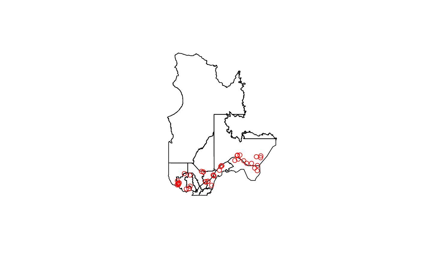
Paginating results
By default, the function paginates the results using a number of
500,000 rows per page, as prescribed by .page_limit default
value. If the table contains more, the function will automatically
download the results in multiple pages and concatenate them into a
single data frame.
You can customize the pagination behavior by specifying the limit and offset parameters in the query. The db_read_table() function also provides additional parameters to control the pagination process, such as .n_pages and .page_limit.
Here’s an example of how to use the get_table_data() function to download the 100 rows of a table, starting at row 200:
data <- db_read_table("taxa_obs", schema = "public", limit = 100, offset = 200)In this example, the results are paginated into multiple pages of 100 rows each.
data <- db_read_table("taxa_obs", schema = "public", .page_limit = 100)Parallelization of Requests
To handle downloading data with very large number of rows, the
function makes requests in parallel using multiple cores. The
db_read_table() function provides an optional parameter,
.cores, to specify the number of cores to use for parallel
processing.
By default, the function downloads the results using parallelization
using 4 cores, as defined by default value of .cores. The
function will automatically determine the number of pages to download
and split the work across the specified number of cores. The results are
then combined into a single data frame.
Here’s an example of how to use the db_read_table() function to download four pages of data in parallel using 4 cores:
data <- db_read_table("observations", schema = "public", .n_pages = 4, .cores = 4)Reading functions data
The db_call_function() function is used to read data from a
PostgreSQL function. It takes several arguments, including the name of
the function, the schema that the function belongs to, and the
authentication token that is required to access the database. Functions
arguments can be passed to the function using the ...
argument.
Accepted arguments are described in the function documentation. For
example, the atlas_api.obs_summary function takes the
following optionnal arguments (taxa_keys,
min_year, max_year, region_fid,
region_type).
data <- db_call_function("obs_summary", schema = "atlas_api")
head(data)
#> # A tibble: 1 × 13
#>     fid count_datasets obs_count taxa_count taxa_count_carrousel taxa_id_list
#>   <int>          <int>     <int>      <int>                <int> <list>
#> 1     1            826  44583587      27117                41219 <int [41,219]>
#> # ℹ 7 more variables: carrousel_info <list>,
#> #   taxa_filter_tags.taxa_tags_fr <lgl>, taxa_filter_tags.taxa_tags_en <lgl>,
#> #   region_filter_tags.tags_fr <chr>, region_filter_tags.tags_en <chr>,
#> #   region_filter_tags.name_fr <chr>, region_filter_tags.name_en <chr>

data <- db_call_function("obs_summary", schema = "atlas_api", taxa_keys = c(1, 2, 3), min_year = 2010, max_year = 2015, region_fid = 1, region_type = 'admin')
head(data)
#> # A tibble: 1 × 13
#>     fid count_datasets obs_count taxa_count taxa_count_carrousel taxa_id_list
#>   <int>          <int>     <int>      <int>                <int> <list>
#> 1     1              1         4          1                    1 <int [1]>
#> # ℹ 7 more variables: carrousel_info <list>,
#> #   taxa_filter_tags.taxa_tags_fr <list>, taxa_filter_tags.taxa_tags_en <list>,
#> #   region_filter_tags.tags_fr <chr>, region_filter_tags.tags_en <chr>,
#> #   region_filter_tags.name_fr <chr>, region_filter_tags.name_en <chr>